
Sunday, August 17, 2025 | 9 minutes
Visualising Decision Trees
I’ve seen lots on how decision trees work, but often the descriptions are textual. I’m a visual person, so let’s do a visual exploration.
The code for this little project is available in my GitHub here: https://github.com/jamesdeluk/data-projects/tree/main/visualising-trees
I’m not going to talk about how the splits are done mathematically (i.e. how they minimise MAE/MSE for regression models, or how they calculate Gini impurity or entropy for classification models); this is more from the use-case perspective, understanding the impact of different hyperparameters on getting the result you want.
Setting up
I’m going to use scikit-learn’s DecisionTreeRegressor. From the hyperparameter persepctive, classification decision trees work similarly to regression ones, so I won’t discuss them separately.
I’m going to use the California housing dataset, available through scikit-learn. It looks something like this:
| MedInc | HouseAge | AveRooms | AveBedrms | Population | AveOccup | Latitude | Longitude | MedHouseVal |
|---|---|---|---|---|---|---|---|---|
| 8.3252 | 41 | 6.98412698 | 1.02380952 | 322 | 2.55555556 | 37.88 | -122.23 | 4.526 |
| 8.3014 | 21 | 6.23813708 | 0.97188049 | 2401 | 2.10984183 | 37.86 | -122.22 | 3.585 |
| 7.2574 | 52 | 8.28813559 | 1.07344633 | 496 | 2.80225989 | 37.85 | -122.24 | 3.521 |
| 5.6431 | 52 | 5.8173516 | 1.07305936 | 558 | 2.54794521 | 37.85 | -122.25 | 3.413 |
| 3.8462 | 52 | 6.28185328 | 1.08108108 | 565 | 2.18146718 | 37.85 | -122.25 | 3.422 |
Each row is a “block group”, a geographical area. The columns are, in order: median income, median house age, average number of rooms, average number of bedrooms, population, average number of occupants, latitude, longitude, and the median house value (the target). The target values range from 0.15 to 5.00, with a mean of 2.1.
I set aside the last item to use as my own personal tester:
| MedInc | HouseAge | AveRooms | AveBedrms | Population | AveOccup | Latitude | Longitude | MedHouseVal |
|---|---|---|---|---|---|---|---|---|
| 2.3886 | 16 | 5.25471698 | 1.16226415 | 1387 | 2.61698113 | 39.37 | -121.24 | 0.894 |
I’ll use train_test_split to create training and testing data, which I’ll use to compare the trees.
Tree depth
Shallow
I’ll start with a small tree, with max_depth of 3. I’ll use timeit to record how long it takes to fit and predict. To get a more accurate timing, I took the mean of 10 fit-and-predicts.
It took 0.024s to fit, 0.0002 to predict, and resulted in a mean absolute error (MAE) of 0.6, a mean absolute percentage error (MAPE) of 0.38 (i.e. 38%), a mean squared error (MSE) of 0.65, a root mean squared error (RMSE) of 0.80, and an R² of 0.50. Note that for R², unlike the previous error stats, the higher the better. For my chosen block, it predicted 1.183, vs 0.894 actual. Overall, not great.
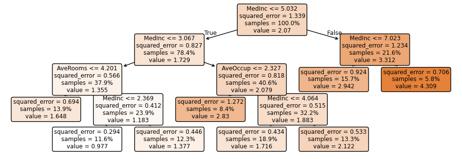
This is the tree itself, using plot_tree:
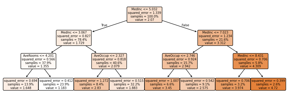
You can see it only uses the MedInc, AveRooms, and AveOccup features - in other words, removing HouseAge, AveBedrms, Population, Latitude, and Longitude from the dataset would give the same predictions.
Deep
Let’s go to max_depth of None, i.e. unlimited.
It took 0.09s to fit (~4x longer), 0.0007 to predict (~4x longer), and resulted in an MAE of 0.47, an MAPE of 0.26, an MSE of 0.53, an RMSE of 0.73, and an R² of 0.60. For my chosen block, it predicted 0.819, vs 0.894 actual. Much better.
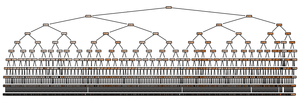
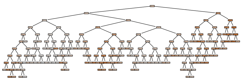
The tree:
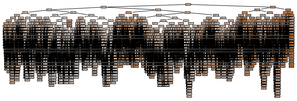
Wow. It has 34 levels (.get_depth()), 29,749 nodes (.tree_.node_count), and 14,875 individual branches (.get_n_leaves()) - in other words, up to 14,875 different final values for MedHouseVal.
Using some custom code, I can plot one of the branches:
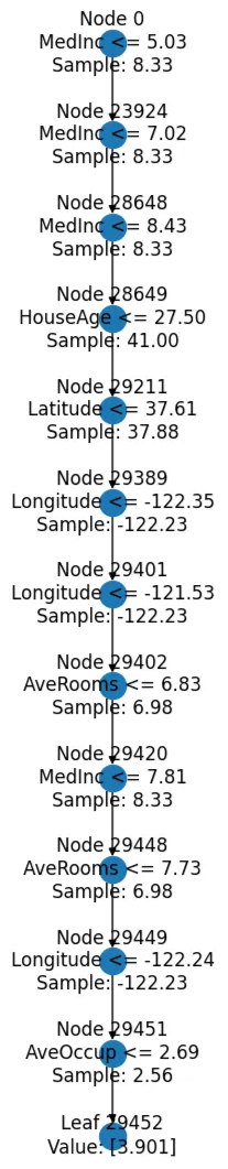
This branch alone uses six of the eight features, so it’s likely that, across all ~15,000 branches, all features are represented.
However, a tree this complex can lead to overfitting, as it can split into very small groups and capture noise.
Pruned
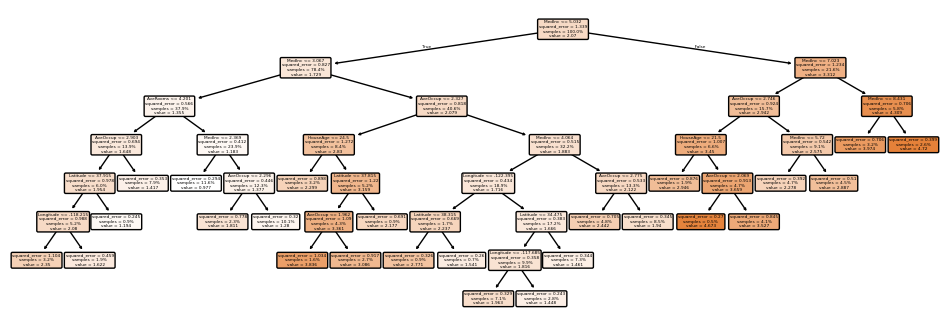
The ccp_alpha parameter (ccp = cost-complexity pruning) can prune a tree after it’s built. Adding in a value of 0.005 to the unlimited depth tree results in an MAE of 0.53, an MAPE of 0.33, an MSE of 0.52, an RMSE of 0.72, and an R² of 0.60 - so it performed between the deep and shallow trees. For my chosen block, it predicted 1.279, so in this case, worse than the shallow one. It took 0.64s to fit (>6x longer than the deep tree) and 0.0002 to predict (the same as the shallow tree) - so, it’s slow to fit, but fast to predict.
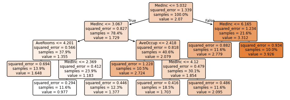
This tree looks like:
Cross validating
What if we mix up the data? Within a loop, I used train_test_split without a random state (to get new data each time), and fitted and predicted each tree based on the new data. Every loop I recorded the MAE/MAPE/MSE/RMSE/R², and then found the mean and standard deviation for each. I did 1000 loops. This helps (as the name suggests) validate our results - a single high or low error result could simply be a fluke, so taking the mean gives a better idea of the typical error on new data, and the standard deviation helps understand how stable/reliable a model is.
It’s worth noting that sklearn has some built-in tools for this form of validation, namely cross_validation, using ShuffleSplit or RepeatedKFold, and they’re typically much faster; I just did it manually to make it clearer what was going on, and to emphasise the time difference.
max_depth=3 (time: 22.1s)
| Metric | Mean | Std |
|---|---|---|
| MAE | 0.597 | 0.007 |
| MAPE | 0.378 | 0.008 |
| MSE | 0.633 | 0.015 |
| RMSE | 0.795 | 0.009 |
| R² | 0.524 | 0.011 |
max_depth=None (time: 100.0s)
| Metric | Mean | Std |
|---|---|---|
| MAE | 0.463 | 0.010 |
| MAPE | 0.253 | 0.008 |
| MSE | 0.524 | 0.023 |
| RMSE | 0.724 | 0.016 |
| R² | 0.606 | 0.018 |
max_depth=None, ccp_alpha=0.005 (time: 650.2s)
| Metric | Mean | Std |
|---|---|---|
| MAE | 0.531 | 0.012 |
| MAPE | 0.325 | 0.012 |
| MSE | 0.521 | 0.021 |
| RMSE | 0.722 | 0.015 |
| R² | 0.609 | 0.016 |
Compared with the deep tree, across all error stats, the shallow tree has higher errors (also known as biases), but lower standard deviations (also known as variances). In more casual terminology, there’s a trade-off between precision (all predictions being close together) and accuracy (all predictions being near the true value). The pruned deep tree generally performed between the two, but took far longer to fit.
We can visualise all the stats these with box plots:
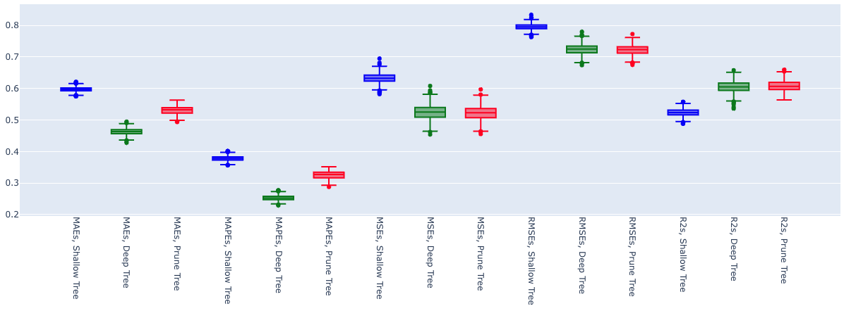
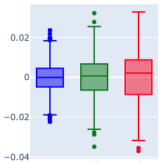
We can see the deep trees (green boxes) typically have lower errors (smaller y-axis value) but larger variations (larger gap between the lines) than the shallow tree (blue boxes). Normalising the means (so they’re all 0), we can see the variation more clearly; for example, for the MAEs:
Histograms can also be interesting. Again for the MAEs:
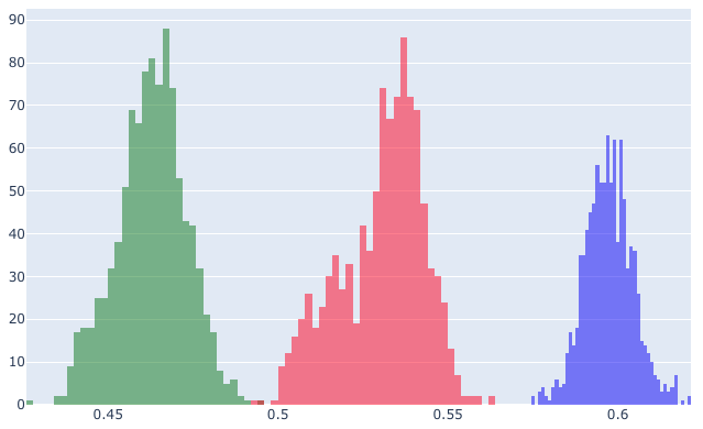
The green (deep) has lower errors, but the blue (shallow) has a narrower band. Interestingly, the pruned tree results are less normal than the other two - although this is not typical behaviour.
Other hyperparameters
What are the other hyperparameters we can tweak? The full list can be found in the docs: https://scikit-learn.org/stable/modules/generated/sklearn.tree.DecisionTreeClassifier.html
Minimum samples to split
This is the minimum number of samples of the total that an individual node can contain to allow splitting. It can be a number or a percentage (implemented as a float between 0 and 1). It helps avoid overfitting by ensure each branch contains a decent number of results, rather than splitting into smaller and smaller branches based on only a few samples.
For example, max_depth=10, which I’ll use as a reference, looks like:
| Metric | Mean | Std |
|---|---|---|
| MAE | 0.426 | 0.010 |
| MAPE | 0.240 | 0.008 |
| MSE | 0.413 | 0.018 |
| RMSE | 0.643 | 0.014 |
| R² | 0.690 | 0.014 |
That’s 1563 nodes and 782 leaves.
Whereas max_depth=10, min_samples_split=0.2 looks like:
| Metric | Mean | Std |
|---|---|---|
| MAE | 0.605 | 0.013 |
| MAPE | 0.367 | 0.007 |
| MSE | 0.652 | 0.027 |
| RMSE | 0.807 | 0.016 |
| R² | 0.510 | 0.019 |
Because it can’t split any node with fewer than 20% (0.2) of the total samples (as you can see in the leaves samples %), it’s limited to a depth of 4, with only 15 nodes and 8 leaves.
For the tree with depth 10, many of the leaves contained a single sample. Having so many leaves with so few sample can be a sign of overfitting. For the constrained tree, the smallest leaf contains over 1000 samples.
In this case, the constrained tree is worse than the unconstrained tree on all counts; however, setting min_samples_split to 10 (i.e. 10 samples, not 10%) improved the results:
| Metric | Mean | Std |
|---|---|---|
| MAE | 0.425 | 0.009 |
| MAPE | 0.240 | 0.008 |
| MSE | 0.407 | 0.017 |
| RMSE | 0.638 | 0.013 |
| R² | 0.695 | 0.013 |
This one was back to depth 10, with 1133 nodes and 567 leaves (so about 1/3 less than the unconstrained tree). Many of these leaves also contain a single sample.
Minimum samples per leaf
Another way of constraining a tree is by setting a minimum number of samples a leaf can have. Again, this can be a number or a percentage.
With max_depth=10, min_samples_leaf=0.1:
Similar to the first min_samples_split one, it has a depth of 4, 15 nodes, and 8 leaves. However, notice the nodes and leaves are different; for example, in the right-most leaf in the min_samples_split tree, there were 5.8% of the samples, whereas in this one, the “same” leaf has 10% (that’s the 0.1).
The stats are similar to that one also:
| Metric | Mean | Std |
|---|---|---|
| MAE | 0.609 | 0.010 |
| MAPE | 0.367 | 0.007 |
| MSE | 0.659 | 0.023 |
| RMSE | 0.811 | 0.014 |
| R² | 0.505 | 0.016 |
Allowing “larger” leaves can improve results. min_samples_leaf=10 has depth 10, 961 nodes and 481 leaves - so similar to a min_samples_split=10. It gives our best results so far, suggesting limiting the number of 1-sample leaves has indeed reduced overfitting.
| Metric | Mean | Std |
|---|---|---|
| MAE | 0.417 | 0.010 |
| MAPE | 0.235 | 0.008 |
| MSE | 0.380 | 0.017 |
| RMSE | 0.616 | 0.014 |
| R² | 0.714 | 0.013 |
Maximum leaf nodes
Another way to stop having too many leaves with too few samples is to limit the number of leaves directly with max_leaf_nodes (technically it could still result in a single-sample leaf, but it’s less likely). The trees above above varied from 8 to almost 800 leaves. With max_depth=10, max_leaf_nodes=100:
This has a depth of 10 again, with 199 nodes and 100 leaves. In this case, there was only one leaf with a single sample, and only nine of them had fewer than ten samples. The results were decent too:
| Metric | Mean | Std |
|---|---|---|
| MAE | 0.450 | 0.010 |
| MAPE | 0.264 | 0.010 |
| MSE | 0.414 | 0.018 |
| RMSE | 0.644 | 0.014 |
| R² | 0.689 | 0.013 |
Bayes searching
Finally, what’s the “perfect” tree for this data? Sure, it’s possible to use trial-and-error with the above hyperparamters, but it’s much easier to use something like BayesSearchCV (assuming you have the time to let it run). In 20 minutes it performed 200 iterations (i.e. hyperparameter combinations) with five cross-validations (similar to five train_test_splits) each.
The hyperparameters it found: {'ccp_alpha': 0.0, 'criterion': 'squared_error', 'max_depth': 100, 'max_features': 0.9193546958301854, 'min_samples_leaf': 15, 'min_samples_split': 24}.
The tree was depth 20, with 798 leaves and 1595 nodes, so significantly less than the fully deep tree. This clearly demonstrates how increasing min_samples_ can help; while the numbers of leaves and nodes are similar to the depth 10 tree, having “larger” leaves with a deeper tree has improved the results.
For my single block it predicted 0.81632, so pretty close to the true value.
After putting it through the 1000 loops (which took just over 60 seconds - showing that the longest factor when fitting a tree is the pruning), the final scores:
| Metric | Mean | Std |
|---|---|---|
| MAE | 0.393 | 0.007 |
| MAPE | 0.216 | 0.006 |
| MSE | 0.351 | 0.013 |
| RMSE | 0.592 | 0.011 |
| R² | 0.736 | 0.010 |
Adding these to the box plots:
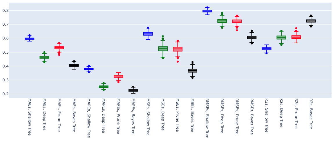
Lower errors, lower variances, and higher R². Excellent.
Next, random forests!